You Need to Know the Formula to Compute Line Integrals Using Parametrization of the Curve.

Show Mobile Discover Show All NotesHibernate All Notes

Mobile Observe

You appear to exist on a device with a "narrow" screen width (i.e. yous are probably on a mobile phone). Due to the nature of the mathematics on this site it is best views in landscape mode. If your device is not in mural fashion many of the equations will run off the side of your device (should be able to scroll to meet them) and some of the bill of fare items will be cut off due to the narrow screen width.

Department 5-ii : Line Integrals - Function I

In this section we are at present going to introduce a new kind of integral. Withal, before we do that it is important to note that y'all will need to recall how to parameterize equations, or put another manner, y'all volition need to be able to write down a fix of parametric equations for a given bend. You should take seen some of this in your Calculus Two course. If you need some review you should go back and review some of the nuts of parametric equations and curves.

Here are some of the more basic curves that we'll demand to know how to practice every bit well as limits on the parameter if they are required.

With the terminal one we gave both the vector form of the equation besides as the parametric course and if nosotros demand the two-dimensional version then we only drop the \(z\) components. In fact, we volition be using the 2-dimensional version of this in this section.

For the ellipse and the circle we've given 2 parameterizations, one tracing out the curve clockwise and the other counter-clockwise. Every bit we'll somewhen see the direction that the bend is traced out can, on occasion, change the reply. Also, both of these "outset" on the positive \(x\)-axis at \(t = 0\).

At present let's motion on to line integrals. In Calculus I we integrated \(f\left( x \right)\), a function of a unmarried variable, over an interval \(\left[ {a,b} \correct]\). In this case nosotros were thinking of \(x\) equally taking all the values in this interval starting at \(a\) and ending at \(b\). With line integrals we will showtime with integrating the function \(f\left( {10,y} \right)\), a office of ii variables, and the values of \(x\) and \(y\) that we're going to use volition be the points, \(\left( {ten,y} \right)\), that lie on a bend \(C\). Note that this is unlike from the double integrals that we were working with in the previous chapter where the points came out of some two-dimensional region.

Let'southward start with the curve \(C\) that the points come from. We will assume that the curve is smooth (defined soon) and is given by the parametric equations,

\[10 = h\left( t \right)\hspace{0.25in}y = g\left( t \right)\hspace{0.25in}\,\,\,\,a \le t \le b\]

We volition oftentimes want to write the parameterization of the curve as a vector function. In this case the curve is given by,

\[\vec r\left( t \right) = h\left( t \right)\,\vec i + g\left( t \right)\vec j\hspace{0.25in}\hspace{0.25in}a \le t \le b\]

The curve is called smooth if \(\vec r'\left( t \right)\) is continuous and \(\vec r'\left( t \right) \ne 0\) for all \(t\).

The line integral of \(f\left( {10,y} \right)\) along \(C\) is denoted by,

\[\int\limits_{C}{{f\left( {x,y} \correct)\,ds}}\]

We use a \(ds\) here to acknowledge the fact that we are moving along the curve, \(C\), instead of the \(x\)-axis (denoted by \(dx\)) or the \(y\)-centrality (denoted by \(dy\)). Because of the \(ds\) this is sometimes chosen the line integral of \(f\) with respect to arc length.

We've seen the note \(ds\) before. If you recall from Calculus II when nosotros looked at the arc length of a bend given by parametric equations we found it to be,

\[L = \int_{{\,a}}^{{\,b}}{{ds}}\,\,,\hspace{0.25in}{\mbox{where }}ds = \sqrt {{{\left( {\frac{{dx}}{{dt}}} \right)}^2} + {{\left( {\frac{{dy}}{{dt}}} \correct)}^2}} \,dt\]

It is no coincidence that we use \(ds\) for both of these problems. The \(ds\) is the same for both the arc length integral and the notation for the line integral.

And then, to compute a line integral we volition catechumen everything over to the parametric equations. The line integral is and so,

\[\int\limits_{C}{{f\left( {ten,y} \correct)\,ds}} = \int_{{\,a}}^{{\,b}}{{f\left( {h\left( t \right),g\left( t \right)} \right)\sqrt {{{\left( {\frac{{dx}}{{dt}}} \right)}^ii} + {{\left( {\frac{{dy}}{{dt}}} \right)}^2}} \,dt}}\]

Don't forget to plug the parametric equations into the function every bit well.

If we utilise the vector class of the parameterization we can simplify the notation up somewhat by noticing that,

\[\sqrt {{{\left( {\frac{{dx}}{{dt}}} \correct)}^2} + {{\left( {\frac{{dy}}{{dt}}} \right)}^2}} = \left\| {\,\vec r'\left( t \correct)} \right\|\]

where \(\left\| {\vec r'\left( t \right)} \right\|\) is the magnitude or norm of \(\vec r'\left( t \correct)\). Using this notation, the line integral becomes,

\[\int\limits_{C}{{f\left( {ten,y} \correct)\,ds}} = \int_{{\,a}}^{{\,b}}{{f\left( {h\left( t \right),g\left( t \right)} \right)\,\,\left\| {\,\vec r'\left( t \right)} \correct\|\,dt}}\]

Notation that as long as the parameterization of the bend \(C\) is traced out exactly once every bit \(t\) increases from \(a\) to \(b\) the value of the line integral will exist contained of the parameterization of the curve.

Let's take a look at an example of a line integral.

Case ane Evaluate \(\displaystyle \int\limits_{C}{{x{y^iv}\,ds}}\) where \(C\) is the right half of the circle,\({ten^two} + {y^2} = sixteen\) traced out in a counter clockwise direction.

Testify Solution

We start need a parameterization of the circle. This is given by,

\[ten = 4\cos t\hspace{0.25in}y = 4\sin t\]

We now need a range of \(t\)'s that will requite the correct half of the circle. The following range of \(t\)'s volition do this.

\[ - \frac{\pi }{two} \le t \le \frac{\pi }{ii}\]

At present, we need the derivatives of the parametric equations and permit's compute \(ds\).

\[\begin{align*}\frac{{dx}}{{dt}} & = - 4\sin t\hspace{0.25in}\hspace{0.25in}\frac{{dy}}{{dt}} = four\cos t\\ ds & = \sqrt {16{{\sin }^ii}t + 16{{\cos }^two}t} \,dt = four\,dt\end{marshal*}\]

The line integral is then,

\[\brainstorm{marshal*}\int\limits_{C}{{x{y^iv}\,ds}} & = \int_{{\, - {\pi }/{2}\;}}^{{\,{\pi }/{2}\;}}{{four\cos t{{\left( {4\sin t} \right)}^4}\left( 4 \right)dt}}\\ & = 4096\int_{{\, - {\pi }/{ii}\;}}^{{\,{\pi }/{2}\;}}{{\cos t\,\,{{\sin }^4}t\,dt}}\\ & = \left. {\frac{{4096}}{5}{{\sin }^5}t} \right|_{ - \frac{\pi }{2}}^{\frac{\pi }{2}}\\ & = \frac{{8192}}{5}\end{align*}\]

Side by side we need to talk about line integrals over piecewise smooth curves. A piecewise smooth curve is any curve that can be written every bit the spousal relationship of a finite number of smooth curves, \({C_1}\),…,\({C_n}\) where the end point of \({C_i}\) is the starting point of \({C_{i + one}}\). Below is an illustration of a piecewise smooth bend.

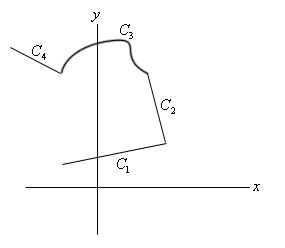
Evaluation of line integrals over piecewise polish curves is a relatively simple thing to do. All we practice is evaluate the line integral over each of the pieces and and then add together them up. The line integral for some part over the above piecewise curve would exist,

\[\int\limits_{C}{{f\left( {x,y} \right)\,ds}} = \int\limits_{{{C_1}}}{{f\left( {x,y} \right)\,ds}} + \int\limits_{{{C_2}}}{{f\left( {10,y} \right)\,ds}} + \int\limits_{{{C_3}}}{{f\left( {x,y} \right)\,ds}} + \int\limits_{{{C_4}}}{{f\left( {x,y} \right)\,ds}}\]

Let's encounter an example of this.

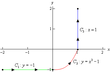
Instance ii Evaluate \(\displaystyle \int\limits_{C}{{four{ten^3}\,ds}}\) where \(C\) is the curve shown below.

Show Solution

So, showtime we need to parameterize each of the curves.

\[\brainstorm{align*}& {C_1}\,\,\,:\,\,\,\,x = t,\,\,y = - i\,,\,\,\,\,\,\,\,\,\,\,\,\, - ii \le t \le 0\\ & {C_2}\,\,:\,\,\,\,\,x = t,\,\,y = {t^3} - 1,\,\,\,\,\,\,\,\,\,\,0 \le t \le 1\\ & {C_3}\,\,:\,\,\,\,\,10 = 1,\,\,\,y = t,\,\,\,\,\,\,\,\,\,\,\,\,\,\,\,\,\,\,\,0 \le t \le 2\cease{align*}\]

At present let'south do the line integral over each of these curves.

\[\int\limits_{{{C_1}}}{{4{10^3}\,ds}} = \int_{{\, - 2}}^{{\,0}}{{4{t^3}\sqrt {{{\left( 1 \right)}^2} + {{\left( 0 \right)}^2}} \,dt}} = \int_{{\, - 2}}^{{\,0}}{{4{t^3}\,dt}} = \left. {{t^iv}} \correct|_{ - 2}^0 = - xvi\] \[\begin{align*}\int\limits_{{{C_2}}}{{4{x^3}\,ds}} & = \int_{{\,0}}^{{\,1}}{{4{t^3}\sqrt {{{\left( 1 \correct)}^ii} + {{\left( {iii{t^2}} \right)}^two}} \,dt}}\\ & = \int_{{\,0}}^{{\,1}}{{four{t^3}\sqrt {1 + ix{t^4}} \,dt}}\\ & = \left. {\frac{one}{9}\left( {\frac{ii}{3}} \right){{\left( {1 + 9{t^4}} \right)}^{\frac{3}{two}}}} \correct|_0^i = \frac{two}{{27}}\left( {{{ten}^{\frac{3}{2}}} - 1} \right) = 2.268\stop{align*}\] \[\int\limits_{{{C_3}}}{{4{x^3}\,ds}} = \int_{{\,0}}^{{\,2}}{{4{{\left( i \right)}^3}\sqrt {{{\left( 0 \right)}^2} + {{\left( 1 \right)}^ii}} \,dt}} = \int_{{\,0}}^{{\,two}}{{four\,dt}} = 8\]

Finally, the line integral that nosotros were asked to compute is,

\[\begin{marshal*}\int\limits_{C}{{iv{x^3}\,ds}} & = \int\limits_{{{C_1}}}{{four{10^iii}\,ds}} + \int\limits_{{{C_2}}}{{iv{ten^3}\,ds}} + \int\limits_{{{C_3}}}{{4{10^three}\,ds}}\\ & = - 16 + two.268 + viii\\ & = - 5.732\end{marshal*}\]

Detect that we put direction arrows on the curve in the above example. The management of motility forth a bend may change the value of the line integral every bit we will see in the next department. Besides note that the bend can exist thought of a curve that takes us from the point \(\left( { - 2, - 1} \right)\) to the point \(\left( {1,two} \right)\). Let'due south first see what happens to the line integral if nosotros change the path between these 2 points.

Example three Evaluate \(\displaystyle\int\limits_{C}{{4{ten^3}\,ds}}\) where \(C\) is the line segment from \(\left( { - two, - ane} \right)\) to \(\left( {1,2} \right)\).

Evidence Solution

From the parameterization formulas at the outset of this section we know that the line segment starting at \(\left( { - 2, - 1} \right)\) and ending at \(\left( {1,ii} \right)\) is given by,

\[\begin{align*}\vec r\left( t \correct) & = \left( {one - t} \right)\left\langle { - ii, - 1} \right\rangle + t\left\langle {1,2} \correct\rangle \\ & = \left\langle { - ii + 3t, - 1 + 3t} \right\rangle \terminate{align*}\]

for \(0 \le t \le 1\). This means that the individual parametric equations are,

\[ten = - 2 + 3t\hspace{0.25in}\hspace{0.25in}y = - 1 + 3t\]

Using this path the line integral is,

\[\begin{align*}\int\limits_{C}{{4{x^3}\,ds}} & = \int_{{\,0}}^{{\,1}}{{four{{\left( { - 2 + 3t} \right)}^three}\sqrt {9 + ix} \,dt}}\\ & = 12\sqrt 2 \left( {\frac{i}{{12}}} \right)\left. {{{\left( { - 2 + 3t} \right)}^4}} \right|_0^1\\ & = 12\sqrt 2 \left( { - \frac{five}{iv}} \right)\\ & = - fifteen\sqrt 2 = - 21.213\stop{align*}\]

When doing these integrals don't forget simple Calc I substitutions to avoid having to do things similar cubing out a term. Cubing it out is not that difficult, simply it is more work than a simple substitution.

So, the previous two examples seem to suggest that if nosotros change the path between two points then the value of the line integral (with respect to arc length) will change. While this will happen fairly regularly we tin can't presume that it will e'er happen. In a later department we volition investigate this idea in more detail.

Next, let'south see what happens if nosotros alter the direction of a path.

Instance 4 Evaluate \(\displaystyle \int\limits_{C}{{four{10^3}\,ds}}\) where \(C\) is the line segment from \(\left( {one,2} \right)\) to \(\left( { - ii, - ane} \correct)\).

Show Solution

This one isn't much different, piece of work wise, from the previous instance. Here is the parameterization of the bend.

\[\begin{align*}\vec r\left( t \right) & = \left( {i - t} \correct)\left\langle {ane,two} \correct\rangle + t\left\langle { - 2, - 1} \right\rangle \\ & = \left\langle {i - 3t,2 - 3t} \right\rangle \end{align*}\]

for \(0 \le t \le i\). Remember that nosotros are switching the management of the curve and this will also change the parameterization so we tin can make sure that we first/terminate at the proper point.

Here is the line integral.

\[\begin{marshal*}\int\limits_{C}{{4{10^3}\,ds}} & = \int_{{\,0}}^{{\,1}}{{4{{\left( {1 - 3t} \right)}^3}\sqrt {9 + nine} \,dt}}\\ & = 12\sqrt 2 \left( { - \frac{one}{{12}}} \right)\left. {{{\left( {1 - 3t} \right)}^iv}} \right|_0^one\\ & = 12\sqrt 2 \left( { - \frac{v}{4}} \right)\\ & = - fifteen\sqrt two = - 21.213\terminate{align*}\]

So, it looks like when we switch the direction of the curve the line integral (with respect to arc length) will not change. This will always be true for these kinds of line integrals. However, there are other kinds of line integrals in which this won't be the case. Nosotros will see more examples of this in the next couple of sections so don't get it into your head that changing the direction will never change the value of the line integral.

Before working some other case allow's formalize this idea up somewhat. Allow's suppose that the bend \(C\) has the parameterization \(x = h\left( t \right)\), \(y = m\left( t \right)\). Let's also suppose that the initial signal on the curve is \(A\) and the last indicate on the curve is \(B\). The parameterization \(x = h\left( t \correct)\), \(y = m\left( t \right)\) will then determine an orientation for the bend where the positive management is the direction that is traced out as \(t\) increases. Finally, let \( - C\) be the curve with the same points as \(C\), nonetheless in this case the curve has \(B\) as the initial point and \(A\) every bit the terminal point, once again \(t\) is increasing as we traverse this curve. In other words, given a curve \(C\), the bend \( - C\) is the same curve equally \(C\) except the direction has been reversed.

We then have the following fact about line integrals with respect to arc length.

Fact

\[\int\limits_{C}{{f\left( {x,y} \right)\,ds}} = \int\limits_{{ - C}}{{f\left( {x,y} \right)\,ds}}\]

So, for a line integral with respect to arc length we can change the direction of the curve and not change the value of the integral. This is a useful fact to recollect every bit some line integrals will be easier in one direction than the other.

Now, allow'southward piece of work another example

Example 5 Evaluate \(\displaystyle \int\limits_{C}{{ten\,ds}}\) for each of the post-obit curves.

1. \({C_1}:y = {10^two},\,\,\, - one \le x \le 1\)
2. \({C_2}\): The line segment from \(\left( { - one,1} \right)\) to \(\left( {1,1} \right)\).
3. \({C_3}\): The line segment from \(\left( {1,ane} \right)\) to \(\left( { - 1,ane} \correct)\).

Show All SolutionsHide All Solutions

Bear witness Word

Before working any of these line integrals allow'south find that all of these curves are paths that connect the points \(\left( { - one,i} \right)\) and \(\left( {1,1} \right)\). Also notice that \({C_3} = - {C_2}\) and and then by the fact above these ii should give the same answer.

Here is a sketch of the three curves and note that the curves illustrating \({C_2}\) and \({C_3}\) have been separated a little to prove that they are separate curves in some way fifty-fifty though they are the same line.

a \({C_1}:y = {ten^two},\,\,\, - 1 \le x \le 1\) Prove Solution

Here is a parameterization for this curve.

\[{C_1}:x = t,\,\,y = {t^two},\,\,\, - 1 \le t \le 1\]

Hither is the line integral.

\[\int\limits_{{{C_1}}}{{x\,ds}} = \int_{{\, - 1}}^{{\,1}}{{t\sqrt {1 + 4{t^2}} \,dt}} = \left. {\frac{1}{{12}}{{\left( {i + 4{t^two}} \correct)}^{\frac{3}{2}}}} \right|_{ - ane}^i = 0\]

b \({C_2}\): The line segment from \(\left( { - one,1} \right)\) to \(\left( {1,1} \right)\). Show Solution

There are two parameterizations that we could use here for this curve. The starting time is to utilize the formula we used in the previous couple of examples. That parameterization is,

\[\begin{align*}{C_2}:\vec r\left( t \right) & = \left( {1 - t} \right)\left\langle { - i,1} \right\rangle + t\left\langle {i,ane} \right\rangle \\ & \hspace{0.25in}\,\,{\kern 1pt} = \left\langle {2t - 1,one} \right\rangle \end{align*}\]

for \(0 \le t \le 1\).

Sometimes we have no choice but to use this parameterization. Yet, in this case at that place is a 2nd (probably) easier parameterization. The second one uses the fact that we are really simply graphing a portion of the line \(y = ane\). Using this the parameterization is,

\[{C_2}:10 = t,\,\,y = one,\,\,\, - 1 \le t \le one\]

This will exist a much easier parameterization to apply so we volition use this. Here is the line integral for this curve.

\[\int\limits_{{{C_2}}}{{x\,ds}} = \int_{{\, - 1}}^{{\,1}}{{t\sqrt {1 + 0} \,dt}} = \left. {\frac{1}{2}{t^2}} \right|_{ - 1}^i = 0\]

Note that this time, unlike the line integral we worked with in Examples 2, 3, and 4 we got the same value for the integral despite the fact that the path is different. This will happen on occasion. We should also not expect this integral to be the aforementioned for all paths betwixt these 2 points. At this point all we know is that for these two paths the line integral volition have the same value. Information technology is completely possible that in that location is some other path betwixt these ii points that will give a different value for the line integral.

c \({C_3}\): The line segment from \(\left( {ane,1} \correct)\) to \(\left( { - 1,1} \right)\). Show Solution

Now, according to our fact in a higher place we really don't demand to do annihilation here since nosotros know that \({C_3} = - {C_2}\). The fact tells united states of america that this line integral should be the same every bit the 2d office (i.e. nix). Even so, let's verify that, plus there is a bespeak we need to make hither nigh the parameterization.

Here is the parameterization for this curve.

\[\begin{marshal*}{C_3}:\vec r\left( t \right) & = \left( {1 - t} \right)\left\langle {ane,one} \correct\rangle + t\left\langle { - i,1} \right\rangle \\ & \hspace{0.25in}\,\,{\kern 1pt} = \left\langle {ane - 2t,1} \correct\rangle \cease{align*}\]

for \(0 \le t \le i\).

Note that this time we can't use the second parameterization that we used in part (b) since we need to movement from right to left as the parameter increases and the 2nd parameterization used in the previous role will motion in the reverse direction.

Here is the line integral for this curve.

\[\int\limits_{{{C_3}}}{{ten\,ds}} = \int_{{\,0}}^{{\,one}}{{\left( {1 - 2t} \correct)\sqrt {four + 0} \,dt}} = \left. {two\left( {t - {t^two}} \right)} \right|_0^1 = 0\]

Sure enough we got the same respond as the second part.

To this point in this department we've merely looked at line integrals over a two-dimensional curve. However, there is no reason to restrict ourselves like that. We can do line integrals over three-dimensional curves every bit well.

Let's suppose that the three-dimensional curve \(C\) is given by the parameterization,

\[x = x\left( t \right),\,\hspace{0.25in}y = y\left( t \right)\hspace{0.25in}z = z\left( t \right)\hspace{0.25in}a \le t \le b\]

then the line integral is given by,

\[\int\limits_{C}{{f\left( {x,y,z} \correct)\,ds}} = \int_{{\,a}}^{{\,b}}{{f\left( {x\left( t \correct),y\left( t \correct),z\left( t \right)} \right)\sqrt {{{\left( {\frac{{dx}}{{dt}}} \right)}^2} + {{\left( {\frac{{dy}}{{dt}}} \right)}^2} + {{\left( {\frac{{dz}}{{dt}}} \correct)}^2}} \,dt}}\]

Note that often when dealing with 3-dimensional space the parameterization will exist given as a vector function.

\[\vec r\left( t \right) = \left\langle {x\left( t \right),y\left( t \right),z\left( t \right)} \right\rangle \]

Detect that we changed upward the note for the parameterization a little. Since we rarely apply the role names we simply kept the \(x\), \(y\), and \(z\) and added on the \(\left( t \correct)\) role to denote that they may be functions of the parameter.

Besides notice that, as with two-dimensional curves, nosotros have,

\[\sqrt {{{\left( {\frac{{dx}}{{dt}}} \right)}^2} + {{\left( {\frac{{dy}}{{dt}}} \right)}^2} + {{\left( {\frac{{dz}}{{dt}}} \right)}^2}} = \left\| {\,\vec r'\left( t \right)} \right\|\]

and the line integral can again exist written as,

\[\int\limits_{C}{{f\left( {x,y,z} \right)\,ds}} = \int_{{\,a}}^{{\,b}}{{f\left( {x\left( t \right),y\left( t \correct),z\left( t \right)} \right)\,\,\left\| {\vec r'\left( t \right)} \right\|\,dt}}\]

And so, outside of the addition of a third parametric equation line integrals in iii-dimensional space work the aforementioned as those in two-dimensional space. Let'due south work a quick example.

Example half-dozen Evaluate \(\displaystyle \int\limits_{C}{{xyz\,ds}}\) where \(C\) is the helix given by, \(\vec r\left( t \right) = \left\langle {\cos \left( t \correct),\sin \left( t \right),3t} \right\rangle \), \(0 \le t \le 4\pi \).

Show Solution

Note that we first saw the vector equation for a helix back in the Vector Functions section. Here is a quick sketch of the helix.

Here is the line integral.

\[\brainstorm{align*}\int\limits_{C}{{xyz\,ds}} = \int_{{\,0}}^{{\,four\pi }}{{3t\cos \left( t \right)\sin \left( t \right)\sqrt {{{\sin }^2}t + {{\cos }^2}t + 9} \,dt}}\\ & = \int_{{\,0}}^{{\,4\pi }}{{3t\left( {\frac{1}{2}\sin \left( {2t} \correct)} \correct)\sqrt {1 + 9} \,dt}}\\ & = \frac{{3\sqrt {10} }}{2}\int_{{\,0}}^{{\,4\pi }}{{t\sin \left( {2t} \right)\,dt}}\\ & = \frac{{3\sqrt {10} }}{ii}\left. {\left( {\frac{1}{4}\sin \left( {2t} \right) - \frac{t}{2}\cos \left( {2t} \right)} \right)} \correct|_0^{4\pi }\\ & = - three\sqrt {ten} \,\pi \stop{align*}\]

You were able to practise that integral right? Information technology required integration by parts.

And then, as we can meet at that place really isn't too much departure between two- and iii-dimensional line integrals.

schmidtcaranown.blogspot.com

Source: https://tutorial.math.lamar.edu/classes/calciii/lineintegralspti.aspx

Share this post